Polar ice melt and sea level rise: earth climate in uncharted territory

By distinction from Mars (Temperature -113 C to 0 C ; thin atmosphere pressure of 0.01 Bar at surface; CO2 ~95.3%) or Venus (T~450 C ; 90 Bar at surface; atmosphere of CO2 & sulphuric acid), the modulation of Earth surface temperature by greenhouse gases (GHG) prevents its freezing to -18 C, thus allowing the presence of liquid water and thereby of life.

The connections between the level of GHG, troposphere temperatures, formation or melting of ice and therefore variations is sea level (Figure 1) are in the core of climate science, including future climate projections [1, 2].

Changes in sea level (SL), consequent on the cumulative outcome of thermal expansion or contraction of water and the melting or freezing of ice sheets and mountain glaciers (in the long term SL is also affected by uplift or sinking of continents and ocean floor), represent a definitive measure of variations in Earth climate.

Temperature controlled variations in SL, from +75 meters to -120 meters relative to the present, have resulted in different global land-sea configurations, from flooded Cretaceous (145-65 million years-ago) continents to extended continental shelves during the Pleistocene (1.8-0 m.y.-ago) ice ages (Figures 1, 4).

The measurement of past sea levels from ice core and sediment proxy data and of recent and present levels using tide gauges and laser ranging satellite, allows oceanographers to reconstruct past SL (Figure 1, 4) and near-past SL (Figure 2), demonstrating close connections between atmospheric CO2 levels, temperatures and sea levels (Figure 1, 4).

The data indicate an extreme development in the atmosphere-ocean-cryosphere system since the mid-18^th century, including [1 - 5]:

1. A rise in atmospheric CO2 levels from ~280 ppm prior to 1750 to 391 ppm at present, i.e. near-40% above maximum levels of the last 800,000 years (Figure 1, 4).

2. A concomitant rise in atmospheric methane levels from ~700 to ~1700 parts per billion (ppb).

3. A rise in atmospheric temperatures, most particularly since about 1910 [3], the mean global level rising by 0.56 C between 1975-2009 and polar temperatures rising by between 2 C and 4 C during this period [4], driving sea ice melt (Arctic) and continental ice sheet melt (Greenland, Antarctica).

4. A rise in the rate of sea level rise (1850-1970: ~0.11 cm/year; 1975-2009: ~0.34 cm/year), amounting to a total of ~20 cm since 1870 (Figure 2).

Attempts at estimating future melting of continental ice sheets and thus sea level rise vary between authors. The IPCC-2007 report [2] suggests sea level rise in the range of 0.18-0.59 meter by 2100 but this is qualified by likely underestimate of contributions from ice sheet melt, as ice sheet physics were not understood well enough [1, 2].

Higher estimates followed, including 0.5-1.4 meters above 1990 levels by 2100, assuming a linear proportionally constant rate of 0.34 cm per year per C [5]. Vermeer and Rahmstorf (2009) [7] update their estimate to 0.75-1.9 meters while Alley, 2100 [8] estimates about 1 meter by 2100. Similar-scale estimates are made by Pfeffer et al. 2008 [6] who suggested a possible 0.8 meters and an upper limit of 2.0 meters by 2100.

Note that most projections end by 2100, a time when grandchildren and their children are supposed to live?

In an article titled “Scientific reticence and sea level rise” [9] Hansen et al., 2007, stressing the non-linearity of ice melt processes, state: “as a physicist, I find it almost inconceivable that Business-as Usual climate change would not yield a sea level change of the order of meters on the century timescale”. Most recently Hansen and Sato [1], citing Velicogna, 2009 [10], point to Gravity satellite evidence for a doubling time of about 10 years of Greenland and Antarctic ice melt rates (Figure 3), implying the possibility of multi-meter sea level rise this century.

In a new article Velicogna and Rignot [11], from mass balance calculations and GRACE gravity satellite measurements, report the Greenland and Antarctic ice sheets are losing mass at an accelerated rate, losing a combined mass of 475 billion ton ice per year on average and becoming the dominant contributors to sea level rise. This is consistent with Hansen and Sato’s [1] view of the non-linearity of ice melt dynamic processes reinforced by ice melt feedback processes, rendering multi-meter sea level rise this century possible.

The extreme rate of greenhouse gas forcing, rising at ~2 ppm CO2/year, leads potentially to tipping points such as high-rate methane release from permafrost and Arctic sediments, and the potential collapse of the North Atlantic Thermohaline Stream.

Doubts are often raised among climate scientists whether the Greenland and West Antarctic ice sheets can survive the 1.8 – 4.0 C temperature rises projected by the IPCC-2007 [2], leading to meters-scale sea level rise.

The increase in frequency of extreme weather events manifests a rise in the atmosphere/ocean energy level. Global temperature rise, ice melt and sea level rise lag behind the rise of GHG forcing of about ~2 Watt/m2 [2] (Figure 4). The precise time scale of this lag remains unknown.

The Earth climate is entering uncharted territory.

[1] http://www.columbia.edu/~jeh1/mailings/2011/20110118_MilankovicPaper.pdf

[2] IPCC 2007

[3] http://data.giss.nasa.gov/gistemp/graphs/

[4] http://data.giss.nasa.gov/gistemp/maps/

[5] Rahmstorf et al., 2007. http://www.sciencemag.org/content/315/5810/368.short

[6] Pfeffer et al., 2008. http://climatechangepsychology.blogspot.com/2008/12/w-t-pfeffer-j-t-harper-s-oneel.html

[7] Vermeer and Rahmstorf, 2009. Vermeer: Global sea level linked to global temperature, Proc. Natl.Acad. Sci., 106, 21527-21532.

[8] Alley, 2010. Alley, R.B., 2010: Ice in the hot box—What adaptation challenges might we face? 2010 AGU Fall Meeting, December 17, U52A-02.

[9] Hansen et al., 2007. http://iopscience.iop.org/1748-9326/2/2/024002/fulltext

[10] Velicogna, I., 2009: Increasing rates of ice mass loss from the Greenland and Antarctic ice sheets revealed by GRACE, Geophys. Res. Lett., 36, L19503, doi:10.1029/2009GL040222.

[11] http://www.agu.org/news/press/pr_archives/2011/2011-09.shtml

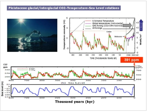
Figure 1.

Variations in CO2, temperatures and sea levels through the 600,000 years of the glacial-interglacial record deduced from Greenland and Antarctic ice cores.

http://www.columbia.edu/~jeh1/mailings/2011/20110118_MilankovicPaper.pdf

The upper diagram plots temperature and radiative forcing anomalies in Watt/m2. Note the increase in radiative forcing by >2 Watt/m2 since the 18^th century. The lower plot correlates CO2 with sea level changes.

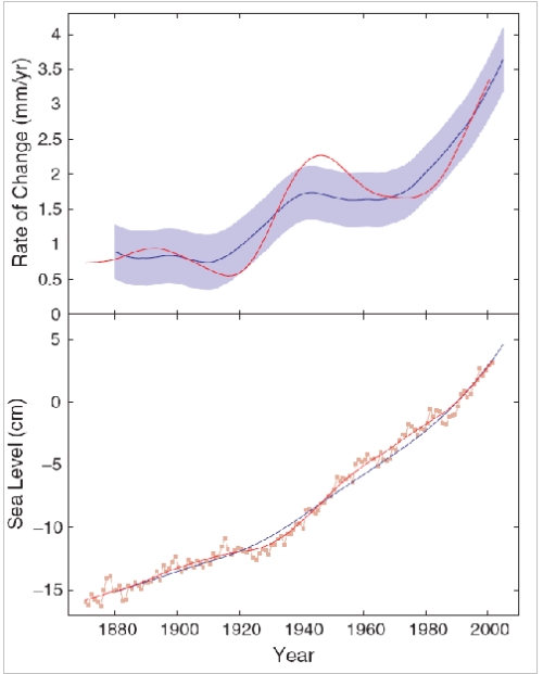
Figure 2.

Rate of sea-level rise obtained from tide gauge observations (red line, smoothed as described in the Fig. 2 legend) and computed from global mean temperature (dark blue line). The light blue band indicates the statistical error (one SD) of the simple linear prediction (upper plot). Sea level relative to 1990 obtained from observations (red line) and computed from global mean temperature (lower plot). The red squares mark the unsmoothed, annual sea-level data [5].

Figure 3.

Greenland (a) and Antarctic (b) mass change deduced from gravitational field measurements by Velicogna (2009), as read by M.Sato from Velicongna’s 2009 graph, and the derivative of these curves, i.e., annual changes of the Greenland (c) and Antarctic (d) ice sheet masses. From Hansen and Sato [1]

Figure 4.

Sea level vs CO2 plot, showing glacial and interglacial data points from Greenland and Antarctic ice cores, values of Earth atmosphere and sea levels during the pre-industrial period, shift of the Earth atmosphere and sea level since the 18^th century (red near-horizontal arrow) and mid-Pliocene (3 m.y.) CO2 and sea level values (red vertical arrow). After [1]..